NumPy Fundamentals: The Backbone of Data Science in Python

numpy day 2

Welcome to the second installment of our Python for Data Science series! In our previous post, we introduced the fundamentals of Python for data science. Today, we're diving into NumPy, the foundational library that powers nearly all of Python's data science ecosystem.

Why NumPy Matters

NumPy (Numerical Python) may not be as flashy as machine learning libraries, but it serves as the foundation upon which libraries like Pandas, Scikit-learn, and TensorFlow are built. Understanding NumPy will give you powerful tools for data manipulation and provide deeper insight into how other libraries work behind the scenes.

Key reasons NumPy is essential:

• Performance: NumPy operations are significantly faster than equivalent Python code

• Memory efficiency: Arrays use less memory than Python lists

• Vectorization: Perform operations on entire arrays without explicit loops

• Scientific computing: Built-in functions for linear algebra, Fourier transforms, and more

Getting Started with NumPy

Let's begin with the basics: installing and importing NumPy.

python

# If you haven't installed NumPy yet
# pip install numpy

# Import NumPy with the standard alias
import numpy as np

NumPy Arrays: The Building Blocks

At the core of NumPy is the ndarray (N-dimensional array) object. Unlike Python lists, NumPy arrays have a fixed size and contain elements of the same type, which enables more efficient operations.

Creating Arrays

There are multiple ways to create NumPy arrays:

python

# From Python lists
basic_array = np.array([1, 2, 3, 4, 5])
print(basic_array)  # [1 2 3 4 5]

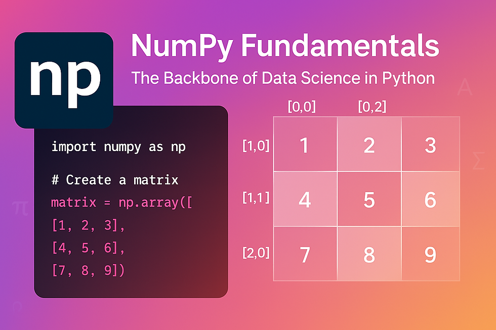
# 2D array (matrix)
matrix = np.array([[1, 2, 3], [4, 5, 6], [7, 8, 9]])
print(matrix)
# [[1 2 3]
#  [4 5 6]
#  [7 8 9]]

# Arrays with specific values
zeros = np.zeros((3, 4))  # 3x4 array of zeros
ones = np.ones((2, 5))    # 2x5 array of ones
empty = np.empty((2, 3))  # 2x3 uninitialized array

# Sequences
range_array = np.arange(0, 10, 2)  # [0 2 4 6 8]
linear_space = np.linspace(0, 1, 5)  # 5 evenly spaced values from 0 to 1: [0.   0.25 0.5  0.75 1.  ]

# Identity matrix
identity = np.eye(3)
# [[1. 0. 0.]
#  [0. 1. 0.]
#  [0. 0. 1.]]

# Random numbers
random_array = np.random.rand(3, 3)  # 3x3 array of random values between 0 and 1

Array Attributes

NumPy arrays come with useful attributes that provide information about their structure:

python

arr = np.array([[1, 2, 3], [4, 5, 6]])

print(arr.shape)     # (2, 3) - dimensions of the array
print(arr.ndim)      # 2 - number of dimensions
print(arr.size)      # 6 - total number of elements
print(arr.dtype)     # int64 - data type of elements

Array Indexing and Slicing

Efficient data access is crucial for data science. NumPy provides powerful ways to select, extract, and modify array elements.

Basic Indexing

python

arr = np.array([[1, 2, 3, 4], [5, 6, 7, 8], [9, 10, 11, 12]])

# Get a single element
print(arr[0, 0])     # 1
print(arr[2, 3])     # 12

# Get a row
print(arr[1])        # [5 6 7 8]

# Get a column
print(arr[:, 2])     # [3 7 11]

Slicing

Slicing works similar to Python lists but extends to multiple dimensions:

python

arr = np.array([[1, 2, 3, 4], [5, 6, 7, 8], [9, 10, 11, 12]])

# Slice rows and columns
print(arr[0:2, 1:3])
# [[2 3]
#  [6 7]]

# Using steps
print(arr[::2, ::2])
# [[1 3]
#  [9 11]]

Boolean Indexing

One of NumPy's most powerful features is the ability to select elements based on conditions:

python

arr = np.array([1, 2, 3, 4, 5, 6, 7, 8, 9])

# Get all elements greater than 5
print(arr[arr > 5])  # [6 7 8 9]

# Combine conditions
print(arr[(arr > 3) & (arr < 8)])  # [4 5 6 7]

# Apply to multi-dimensional arrays
matrix = np.array([[1, 2, 3], [4, 5, 6], [7, 8, 9]])
print(matrix[matrix > 5])  # [6 7 8 9]

Array Operations

The true power of NumPy comes from its ability to perform operations on entire arrays efficiently.

Element-wise Operations

python

a = np.array([1, 2, 3])
b = np.array([4, 5, 6])

# Addition
print(a + b)        # [5 7 9]
# or
print(np.add(a, b))  # [5 7 9]

# Subtraction
print(a - b)        # [-3 -3 -3]

# Multiplication
print(a * b)        # [4 10 18]

# Division
print(a / b)        # [0.25 0.4  0.5 ]

# Exponentiation
print(a ** 2)       # [1 4 9]

# Functions
print(np.sqrt(a))   # [1.         1.41421356 1.73205081]
print(np.exp(a))    # [ 2.71828183  7.3890561  20.08553692]

Aggregation Functions

NumPy provides functions to compute statistics across array elements:

python

arr = np.array([1, 2, 3, 4, 5])

print(np.sum(arr))      # 15
print(np.mean(arr))     # 3.0
print(np.median(arr))   # 3.0
print(np.min(arr))      # 1
print(np.max(arr))      # 5
print(np.std(arr))      # ~1.41 (standard deviation)

# For multi-dimensional arrays, specify axis
matrix = np.array([[1, 2, 3], [4, 5, 6]])
print(np.sum(matrix, axis=0))  # [5 7 9] (sum of each column)
print(np.sum(matrix, axis=1))  # [6 15] (sum of each row)

Broadcasting

Broadcasting allows NumPy to work with arrays of different shapes when performing arithmetic operations:

python

# Add a scalar to all elements
arr = np.array([1, 2, 3, 4])
print(arr + 10)  # [11 12 13 14]

# More complex broadcasting
a = np.array([[1, 2, 3], [4, 5, 6]])  # 2x3 array
b = np.array([10, 20, 30])            # 1D array with 3 elements

print(a + b)
# [[11 22 33]
#  [14 25 36]]
# Each row of 'a' has the corresponding element of 'b' added to it

Reshaping Arrays

Changing the shape of arrays is a common operation in data preprocessing:

python

arr = np.arange(12)  # [0 1 2 3 4 5 6 7 8 9 10 11]

# Reshape to 3x4 matrix
reshaped = arr.reshape(3, 4)
print(reshaped)
# [[ 0  1  2  3]
#  [ 4  5  6  7]
#  [ 8  9 10 11]]

# Flatten a matrix back to 1D
flattened = reshaped.flatten()
print(flattened)  # [ 0  1  2  3  4  5  6  7  8  9 10 11]

# Transpose a matrix
transposed = reshaped.T
print(transposed)
# [[ 0  4  8]
#  [ 1  5  9]
#  [ 2  6 10]
#  [ 3  7 11]]

Practical Example: Image Processing with NumPy

Let's apply our NumPy knowledge to a real-world example: basic image processing. Images are simply multi-dimensional arrays of pixel values!

python

import numpy as np
import matplotlib.pyplot as plt
from skimage import data  # for sample images

# Load a sample image
astronaut = data.astronaut()
print(f"Image shape: {astronaut.shape}")  # (512, 512, 3) - height, width, RGB channels

# Convert to grayscale - average the RGB channels
grayscale = np.mean(astronaut, axis=2).astype(np.uint8)
print(f"Grayscale shape: {grayscale.shape}")  # (512, 512)

# Create a simple horizontal gradient image
gradient = np.linspace(0, 255, 512).astype(np.uint8)
gradient = np.tile(gradient, (512, 1))  # Repeat the gradient for each row

# Display images
plt.figure(figsize=(12, 4))

plt.subplot(1, 3, 1)
plt.imshow(astronaut)
plt.title('Original')
plt.axis('off')

plt.subplot(1, 3, 2)
plt.imshow(grayscale, cmap='gray')
plt.title('Grayscale')
plt.axis('off')

plt.subplot(1, 3, 3)
plt.imshow(gradient, cmap='gray')
plt.title('Gradient')
plt.axis('off')

plt.tight_layout()
plt.show()

Linear Algebra with NumPy

NumPy provides essential functions for linear algebra operations, which are fundamental to many machine learning algorithms:

python

a = np.array([[1, 2], [3, 4]])
b = np.array([[5, 6], [7, 8]])

# Matrix multiplication
product = np.dot(a, b)
print(product)
# [[19 22]
#  [43 50]]

# Alternative syntax for matrix multiplication
product = a @ b  # Python 3.5+
print(product)
# [[19 22]
#  [43 50]]

# Determinant
det_a = np.linalg.det(a)
print(det_a)  # -2.0

# Inverse
inv_a = np.linalg.inv(a)
print(inv_a)
# [[-2.   1. ]
#  [ 1.5 -0.5]]

# Eigenvalues and eigenvectors
eigenvalues, eigenvectors = np.linalg.eig(a)
print(f"Eigenvalues: {eigenvalues}")
print(f"Eigenvectors: {eigenvectors}")

Practical Tips for Working with NumPy

1. Avoid explicit loops when possible; use vectorized operations for performance.

2. Choose the right data type to save memory (e.g., np.int32 instead of np.int64 for integer arrays).

3. Use views instead of copies when possible to save memory:

   python

   # View (changes affect original array) view = arr[1:3] # Copy (independent from original) copy = arr[1:3].copy()

4. Leverage broadcasting for cleaner code and better performance.

5. Use NumPy's built-in functions instead of writing your own implementations.

Conclusion

NumPy is the cornerstone of the Python data science ecosystem. By mastering NumPy, you've taken a significant step toward becoming proficient in data analysis and machine learning. The concepts you've learned—arrays, indexing, broadcasting, and vectorized operations—will serve as building blocks for more advanced data science techniques.

In our next post, we'll explore Pandas, which builds on NumPy to provide high-level data structures and tools designed specifically for data analysis.

Exercise Challenge

To solidify your NumPy knowledge, try these exercises:

1. Create a 5x5 matrix of random integers between 1 and 100

2. Compute the mean of each row and each column

3. Find all prime numbers in the matrix

4. Replace all even numbers with 0 and all odd numbers with 1

5. Create a 3D array with shape (3, 4, 5) filled with random values and practice slicing it

Post your solutions in the comments, and we'll provide feedback!

What NumPy functions do you find most useful in your data science workflow? Let us know in the comments below!